Over the past few weeks, we’ve started to learn more and more about machine learning and the role it plays in computer vision, image classification, and deep learning.
We’ve seen how Convolutional Neural Networks (CNNs) such as LetNet can be used to classify handwritten digits from the MNIST dataset. We’ve applied the k-NN algorithm to classify whether or not an image contains a dog or a cat. And we’ve learned how to apply hyperparameter tuning to optimize our model to obtain higher classification accuracy.
However, there is another very important machine learning algorithm we have yet to explore — one that can be built upon and extended naturally to Neural Networks and Convolutional Neural Networks.
What is the algorithm?
It’s a simple linear classifier — and while it’s a straightforward algorithm, it’s considered the cornerstone building block of more advanced machine learning and deep learning algorithms.
Keep reading to learn more about linear classifiers and how they can be applied to image classification.
Looking for the source code to this post?
Jump right to the downloads section.
An intro to linear classification with Python
The first half of this tutorial focuses on the basic theory and mathematics surrounding linear classification — and in general — parameterized classification algorithms that actually “learn” from their training data.
From there, I provide an actual linear classification implementation and example using the scikit-learn library that can be used to classify the contents of an image.
4 components of parametrized learning and linear classifiers
I’ve used the word “parameterized” a few times now, but what exactly does it mean?
Simply put: parameterization is the process of defining the necessary parameters of a given model.
In the task of machine learning, parameterization involves defining our problem in terms of:
- Data: This is our input data that we are going to learn from. This data includes both the data points (e.x., feature vectors, color histograms, raw pixel intensities, etc.) and their associated class labels.
- Score function: A function that accepts our data as input and maps the data to class labels. For instance, given our input feature vectors, the score function takes these data points, applies some function f (our score function), and then returns the predicted class labels.
- Loss function: A loss function quantifies how well our predicted class labels agree with our ground-truth labels. The higher level of agreement between these two sets of labels, the lower our loss (and higher our classification accuracy, at least on the training data). Our goal is to minimize our loss function, thereby increasing our classification accuracy.
- Weight matrix: The weight matrix, typically denoted as W, is called the weights or parameters of our classifier that we’ll actually be optimizing. Based on the output of our score function and loss function, we’ll be tweaking and fiddling with the values of our weight matrix to increase classification accuracy.
Note: Depending on your type of model, there may exist many more parameters. But at the most basic level, these are the 4 building blocks of parameterized learning that you’ll commonly see.
Once we’ve defined these 4 key components, we can then apply optimization methods that allow us to find a set of parameters W that minimize our loss function with respect to our score function (while increasing classification accuracy on the data).
Next, we’ll look at how these components work together to build a linear classifier, transforming the input data into actual predictions.
Linear classification: from images to labels
In this section, we are going to look at a more mathematical motivation of the parameterized model to machine learning.
To start we need our data. Let’s assume that our training dataset (either of images or extracted feature vectors) is denoted as  where each image/feature vector has an associated class label
  . We’ll assume
  and
and  implying that we have N data points of dimensionality D (the “length” of the feature vector), separated into K unique categories.
To make this more concrete, consider our previous tutorial on using the k-NN classifier to recognize dogs and cats in images based on extracted color histograms.
This this dataset, we have N = 25,000 total images. Each image is characterized by a 3D color histogram with 8 bins per channel, respectively. This yields a feature vector with D = 8 x 8 x 8 = 512 entries. Finally, we know there are a total of K = 2 class labels, one for the “dog” class and another for the “cat” class.
Given these variables, we must now define a score function f that maps the feature vectors to the class label scores. As the title of this blog post suggests, we’ll be using a simple linear mapping:
 = Wx_{i} + b")
We’ll assume that each is represented as a single column vector with shape [D x 1]. Again, in this example, we’ll be using color histograms — but if we were utilizing raw pixel intensities, we can simply flatten the pixels of the image into a single vector.
Our weight matrix W has a shape of [K x D] (the number of class labels by the dimensionality of the feature vector).
Finally, b, the bias vector is of size [K x 1]. The bias vector essentially allows us to “shift” our scoring function in one direction or another, without actually influencing our weight matrix W — this is often critical for successful learning.
Going back to the Kaggle Dogs vs. Cats example, each is represented by a 512-d color histogram, so therefore has the shape [512 x 1]. The weight matrix W will have a shape of [2 x 512] and finally the bias vector b a size of [2 x 1].
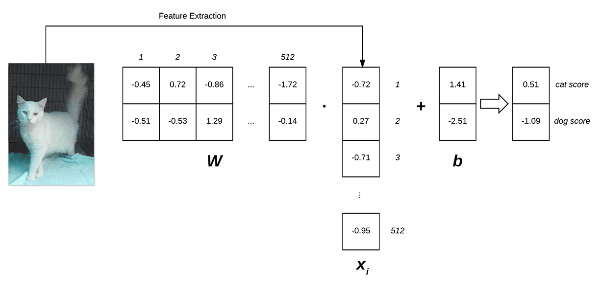
Below follows an illustration of the linear classification scoring function f:
Figure 1: Illustrating the dot product of weight matrix W and feature vector x, followed by addition of the bias term. (Inspired by Karpathy’s example in the CS231n course).
On the left, we have our original input image, which we extract features from. In this example, we’re computing a 512-d color histogram, but any other feature representation could be used (including the raw pixel intensities themselves), but in this case, we’ll simply use a color distribution — this histogram is our representation.
We then have our weight matrix W, which contains 2 rows (one for each class label) and 512 columns (one for each of the entries in the feature vector).
After taking the dot product between  and , we add in the bias vector
  , which has a shape of [2 x 1].
Finally, this yields two values on the right: the scores associated with the dog and cat labels, respectively.
Looking at the above equation, you can convince yourself that the input and are fixed and not something we can modify. Sure, we can obtain different ‘s by applying a different feature extraction technique — but once the features are extracted, these values do not change.
In fact, the only parameters that we have any control over are our weight matrix W and our bias vector b. Therefore, our goal is to utilize both our scoring function and loss function to optimize (i.e., modify) the weight and bias vectors such that our classification accuracy increases.
Exactly how we optimize the weight matrix depends on our loss function, but typically involves some form of gradient descent — we’ll be reviewing optimization and loss functions in a future blog post, but for the time being, simply understand that given a scoring function, we also define a loss function that tells us how “good” our predictions are on the input data.
Advantages of parametrized learning and linear classification
There are two primary advantages to utilizing parameterized learning, such as in the approach I detailed above:
- Once we are done training our model, we can discard the input data and keep only the weight matrix W and the bias vector b. This substantially reduces the size of our model since we only need to store two sets of vectors (versus the entire training set).
- Classifying new test data is fast. In order to perform a classification, all we need to do is take the dot product of
 and
and  , followed by adding in the bias
  . Doing this is substantially faster than needing to compare each testing point to every training example (as in the k-NN algorithm).
Now that we understand linear classification, let’s see how we can implement it in Python, OpenCV, and scikit-learn.
Linear classification of images with Python, OpenCV, and scikit-learn
Much like in our previous example on the Kaggle Dogs vs. Cats dataset and the k-NN algorithm, we’ll be extracting color histograms from the dataset; however, unlike the previous example, we’ll be using a linear classifier rather than k-NN.
Specifically, we’ll be using a Linear Support Vector Machine (SVM) which constructs a maximum-margin separating hyperplane between data classes in an n-dimensional space. The goal of this separating hyperplane is to place all examples (or as many as possible, given some tolerance) of class i on one side of the hyperplane and then all examples not of class i on the other side of the hyperplane.
A detailed description of how Support Vector Machines work is outside the scope of this blog post (but is covered inside the PyImageSearch Gurus course).
In the meantime, simply understand that our Linear SVM utilizes a score function f similar to the one in the “Linear classification: from images to class labels” section of this blog post and then applies a loss function that is used to determine the maximum-margin separating hyperplane to classify the data points (again, we’ll be looking at loss functions in future blog posts).
To get started, open up a new file, name it
linear_classifier.py, and insert the following code:
# import the necessary packages
from sklearn.preprocessing import LabelEncoder
from sklearn.svm import LinearSVC
from sklearn.metrics import classification_report
from sklearn.cross_validation import train_test_split
from imutils import paths
import numpy as np
import argparse
import imutils
import cv2
import os
Lines 2-111 handle importing our required Python packages. We’ll be making use of the scikit-learn library, so if you do not already have it installed, make sure you follow these instructions to get it setup on your machine.
We’ll also be using my imutils Python package, a set of image processing convenience functions. If you do not already have
imutilsinstalled, just let
pipinstall it for you:
$ pip install imutils
We’ll now define our
extract_color_histogramfunction which will be used to extract and quantify the contents of our input images:
# import the necessary packages
from sklearn.preprocessing import LabelEncoder
from sklearn.svm import LinearSVC
from sklearn.metrics import classification_report
from sklearn.cross_validation import train_test_split
from imutils import paths
import numpy as np
import argparse
import imutils
import cv2
import os

def extract_color_histogram(image, bins=(8, 8, 8)):
	# extract a 3D color histogram from the HSV color space using
	# the supplied number of `bins` per channel
	hsv = cv2.cvtColor(image, cv2.COLOR_BGR2HSV)
	hist = cv2.calcHist([hsv], [0, 1, 2], None, bins,
		[0, 180, 0, 256, 0, 256])

	# handle normalizing the histogram if we are using OpenCV 2.4.X
	if imutils.is_cv2():
		hist = cv2.normalize(hist)

	# otherwise, perform "in place" normalization in OpenCV 3 (I
	# personally hate the way this is done
	else:
		cv2.normalize(hist, hist)

	# return the flattened histogram as the feature vector
	return hist.flatten()
This function accepts an input
image, converts it to the HSV color space, and then computes a 3D color histogram using the supplied number of
binsfor each channel.
After computing the color histogram using the
cv2.calcHistfunction, the histogram is normalized and then returned to the calling function.
For a more detailed review of the
extract_color_histogrammethod, please refer to this blog post.
Next, let’s parse our command line arguments and initialize a few variables:
# import the necessary packages
from sklearn.preprocessing import LabelEncoder
from sklearn.svm import LinearSVC
from sklearn.metrics import classification_report
from sklearn.cross_validation import train_test_split
from imutils import paths
import numpy as np
import argparse
import imutils
import cv2
import os

def extract_color_histogram(image, bins=(8, 8, 8)):
	# extract a 3D color histogram from the HSV color space using
	# the supplied number of `bins` per channel
	hsv = cv2.cvtColor(image, cv2.COLOR_BGR2HSV)
	hist = cv2.calcHist([hsv], [0, 1, 2], None, bins,
		[0, 180, 0, 256, 0, 256])

	# handle normalizing the histogram if we are using OpenCV 2.4.X
	if imutils.is_cv2():
		hist = cv2.normalize(hist)

	# otherwise, perform "in place" normalization in OpenCV 3 (I
	# personally hate the way this is done
	else:
		cv2.normalize(hist, hist)

	# return the flattened histogram as the feature vector
	return hist.flatten()

# construct the argument parse and parse the arguments
ap = argparse.ArgumentParser()
ap.add_argument("-d", "--dataset", required=True,
	help="path to input dataset")
args = vars(ap.parse_args())

# grab the list of images that we'll be describing
print("[INFO] describing images...")
imagePaths = list(paths.list_images(args["dataset"]))

# initialize the data matrix and labels list
data = []
labels = []
Lines 33-36 parse our command line arguments. We only need a single switch here,
--dataset, which is the path to our input Kaggle Dogs vs. Cats dataset.
We then grab the
imagePathsto where each of the 25,000 images reside on disk, followed by initializing a
datamatrix to store our extracted feature vectors along with our class
labels.
Speaking of extracting features, let’s go ahead and do that:
# import the necessary packages
from sklearn.preprocessing import LabelEncoder
from sklearn.svm import LinearSVC
from sklearn.metrics import classification_report
from sklearn.cross_validation import train_test_split
from imutils import paths
import numpy as np
import argparse
import imutils
import cv2
import os

def extract_color_histogram(image, bins=(8, 8, 8)):
	# extract a 3D color histogram from the HSV color space using
	# the supplied number of `bins` per channel
	hsv = cv2.cvtColor(image, cv2.COLOR_BGR2HSV)
	hist = cv2.calcHist([hsv], [0, 1, 2], None, bins,
		[0, 180, 0, 256, 0, 256])

	# handle normalizing the histogram if we are using OpenCV 2.4.X
	if imutils.is_cv2():
		hist = cv2.normalize(hist)

	# otherwise, perform "in place" normalization in OpenCV 3 (I
	# personally hate the way this is done
	else:
		cv2.normalize(hist, hist)

	# return the flattened histogram as the feature vector
	return hist.flatten()

# construct the argument parse and parse the arguments
ap = argparse.ArgumentParser()
ap.add_argument("-d", "--dataset", required=True,
	help="path to input dataset")
args = vars(ap.parse_args())

# grab the list of images that we'll be describing
print("[INFO] describing images...")
imagePaths = list(paths.list_images(args["dataset"]))

# initialize the data matrix and labels list
data = []
labels = []

# loop over the input images
for (i, imagePath) in enumerate(imagePaths):
	# load the image and extract the class label (assuming that our
	# path as the format: /path/to/dataset/{class}.{image_num}.jpg
	image = cv2.imread(imagePath)
	label = imagePath.split(os.path.sep)[-1].split(".")[0]

	# extract a color histogram from the image, then update the
	# data matrix and labels list
	hist = extract_color_histogram(image)
	data.append(hist)
	labels.append(label)

	# show an update every 1,000 images
	if i > 0 and i % 1000 == 0:
		print("[INFO] processed {}/{}".format(i, len(imagePaths)))
On Line 47 we start looping over our input
imagePaths. For each
imagePath, we load the
imagefrom disk, extract the class
label, and then quantify the image by computing a color histogram. We then update our
dataand
labelslists, respectively.
Currently, our
labelslist is represented as a list of strings, either “dog” or “cat”. However, many machine learning algorithms in scikit-learn prefer that the
labelsare encoded as integers, with one unique integer per class label.
Performing this conversion of class label string-to-integer is easy with the
LabelEncoderclass:
# import the necessary packages
from sklearn.preprocessing import LabelEncoder
from sklearn.svm import LinearSVC
from sklearn.metrics import classification_report
from sklearn.cross_validation import train_test_split
from imutils import paths
import numpy as np
import argparse
import imutils
import cv2
import os

def extract_color_histogram(image, bins=(8, 8, 8)):
	# extract a 3D color histogram from the HSV color space using
	# the supplied number of `bins` per channel
	hsv = cv2.cvtColor(image, cv2.COLOR_BGR2HSV)
	hist = cv2.calcHist([hsv], [0, 1, 2], None, bins,
		[0, 180, 0, 256, 0, 256])

	# handle normalizing the histogram if we are using OpenCV 2.4.X
	if imutils.is_cv2():
		hist = cv2.normalize(hist)

	# otherwise, perform "in place" normalization in OpenCV 3 (I
	# personally hate the way this is done
	else:
		cv2.normalize(hist, hist)

	# return the flattened histogram as the feature vector
	return hist.flatten()

# construct the argument parse and parse the arguments
ap = argparse.ArgumentParser()
ap.add_argument("-d", "--dataset", required=True,
	help="path to input dataset")
args = vars(ap.parse_args())

# grab the list of images that we'll be describing
print("[INFO] describing images...")
imagePaths = list(paths.list_images(args["dataset"]))

# initialize the data matrix and labels list
data = []
labels = []

# loop over the input images
for (i, imagePath) in enumerate(imagePaths):
	# load the image and extract the class label (assuming that our
	# path as the format: /path/to/dataset/{class}.{image_num}.jpg
	image = cv2.imread(imagePath)
	label = imagePath.split(os.path.sep)[-1].split(".")[0]

	# extract a color histogram from the image, then update the
	# data matrix and labels list
	hist = extract_color_histogram(image)
	data.append(hist)
	labels.append(label)

	# show an update every 1,000 images
	if i > 0 and i % 1000 == 0:
		print("[INFO] processed {}/{}".format(i, len(imagePaths)))

# encode the labels, converting them from strings to integers
le = LabelEncoder()
labels = le.fit_transform(labels)
After the
.fit_transformmethod is called, our
labelsare now represented as a list of integers.
Our final code block will handle partitioning our data into training/testing splits, followed by training our Linear SVM and evaluating it:
# import the necessary packages
from sklearn.preprocessing import LabelEncoder
from sklearn.svm import LinearSVC
from sklearn.metrics import classification_report
from sklearn.cross_validation import train_test_split
from imutils import paths
import numpy as np
import argparse
import imutils
import cv2
import os

def extract_color_histogram(image, bins=(8, 8, 8)):
	# extract a 3D color histogram from the HSV color space using
	# the supplied number of `bins` per channel
	hsv = cv2.cvtColor(image, cv2.COLOR_BGR2HSV)
	hist = cv2.calcHist([hsv], [0, 1, 2], None, bins,
		[0, 180, 0, 256, 0, 256])

	# handle normalizing the histogram if we are using OpenCV 2.4.X
	if imutils.is_cv2():
		hist = cv2.normalize(hist)

	# otherwise, perform "in place" normalization in OpenCV 3 (I
	# personally hate the way this is done
	else:
		cv2.normalize(hist, hist)

	# return the flattened histogram as the feature vector
	return hist.flatten()

# construct the argument parse and parse the arguments
ap = argparse.ArgumentParser()
ap.add_argument("-d", "--dataset", required=True,
	help="path to input dataset")
args = vars(ap.parse_args())

# grab the list of images that we'll be describing
print("[INFO] describing images...")
imagePaths = list(paths.list_images(args["dataset"]))

# initialize the data matrix and labels list
data = []
labels = []

# loop over the input images
for (i, imagePath) in enumerate(imagePaths):
	# load the image and extract the class label (assuming that our
	# path as the format: /path/to/dataset/{class}.{image_num}.jpg
	image = cv2.imread(imagePath)
	label = imagePath.split(os.path.sep)[-1].split(".")[0]

	# extract a color histogram from the image, then update the
	# data matrix and labels list
	hist = extract_color_histogram(image)
	data.append(hist)
	labels.append(label)

	# show an update every 1,000 images
	if i > 0 and i % 1000 == 0:
		print("[INFO] processed {}/{}".format(i, len(imagePaths)))

# encode the labels, converting them from strings to integers
le = LabelEncoder()
labels = le.fit_transform(labels)

# partition the data into training and testing splits, using 75%
# of the data for training and the remaining 25% for testing
print("[INFO] constructing training/testing split...")
(trainData, testData, trainLabels, testLabels) = train_test_split(
	np.array(data), labels, test_size=0.25, random_state=42)

# train the linear regression clasifier
print("[INFO] training Linear SVM classifier...")
model = LinearSVC()
model.fit(trainData, trainLabels)

# evaluate the classifier
print("[INFO] evaluating classifier...")
predictions = model.predict(testData)
print(classification_report(testLabels, predictions,
	target_names=le.classes_))
Lines 70 and 71 handle constructing our training and testing split. We’ll be using 75% of our data for training and the remaining 25% for testing.
To train our Linear SVM, we’ll utilize the
LinearSVCimplementation from the scikit-learn library (Lines 75 and 76).
Finally, we evaluate our classifier on Lines 80-82, displaying a nicely formatted classification report on how well our model performed.
One thing you’ll notice here is that I’m purposely not tuning hyperparameters here, simply to keep this example shorter and easier to digest. However, with that said, I leave tuning the hyperparameters of the
LinearSVCclassifier as an exercise to you, the reader. Use our previous blog post on tuning the hyperparameters of the k-NN classifier as an example.
Evaluating our linear classifier
To test out our linear classifier, make sure you have downloaded:
- The source code to this blog post using the “Downloads” section at the bottom of this tutorial.
- The Kaggle Dogs vs. Cats dataset.
Once you have the code and dataset, you can execute the following command:
$ python linear_classifier.py --dataset kaggle_dogs_vs_cats
The feature extraction process should take approximately 1-3 minutes depending on the speed of your machine.
From there, our Linear SVM is trained and evaluated:
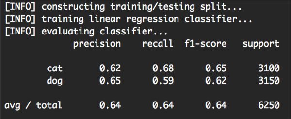
Figure 2: Training and evaluating our linear classifier using Python, OpenCV, and scikit-learn.
As the above figure demonstrates, we were able to obtain 64% classification accuracy, or approximately the same accuracy as using tuned hyperparameters from the k-NN algorithm in this tutorial.
Note: Tuning the hyperparameters to the Linear SVM will lead to a higher classification accuracy — I simply left out this step to make the tutorial a little shorter and less overwhelming.
Furthermore, not only did we obtain the same classification accuracy as k-NN, but our model is much faster at testing time, requiring only a (highly optimized) dot product between the weight matrix and data points, followed by a simple addition.
We are also able to discard the training data after training is complete, leaving us with only the weight matrix W and the bias vector b, leading to a much more compact representation of the classification model.
Summary
In today’s blog post, I discussed the basics of parameterized learning and linear classification. While simple, the linear classifier can be seen as the fundamental building blocks of more advanced machine learning algorithms, extending naturally to Neural Networks and Convolutional Neural Networks.
You see, Convolutional Neural Networks will perform a mapping of raw pixels to class labels similar to what we did in this tutorial — only our score function f will become substantially more complex and contain many more parameters.
A primary benefit of this parameterized approach to learning is that it allows us to discard our training data after our model has been trained. We can then perform classification using only the parameters (i.e., weight matrix and bias vector) learned from the data.
This allows classification to be performed much more efficiently since we: (1) do not need to store a copy of the training data in our model, like in k-NN and (2) we do not need to compare a test image to every training image (an operation that scales O(N), and can become quite cumbersome given many training examples).
In short, this method is significantly faster, requiring only a single dot product and an addition. Pretty neat, right?
Finally, we applied a linear classifier using Python, OpenCV, and scikit-learn to the Kaggle Dogs vs. Cats dataset. After extracting color histograms from the dataset, we trained a Linear Support Vector Machine on the feature vectors and obtained a classification accuracy of 64%, which is fairly reasonable given that (1) color histograms are not the best choice for characterizing dogs vs. cats and (2) we did not tune the hyperparameters to our Linear SVM.
At this point, we are starting to understand the basic building blocks that go into building Neural Networks, Convolutional Neural Networks, and Deep Learning models, but there is still a ways to go.
To start, we need to understand loss functions in more detail, and in particular, how the loss function is used to optimize our weight matrix to obtain more accurate predictions. Future blog posts will go into these concepts in more detail.
Before you go, be sure to sign up for the PyImageSearch Newsletter using the form below to be notified when new blog posts are published!
Downloads:
The post An intro to linear classification with Python appeared first on PyImageSearch.